Tutorial
Dispersion relation finder tutorial
While the graphic interface for the dispersion relation finder is very simple, the use of the program is not entirely intuitive. This tutorial will walk the user through an example in an effort to familiarize him or her with the application’s operation. It will be necessary to download the files at the top of the page in order to follow along. Also, please note that the time required to plot depends on the speed of the computer running it. For a 1 GHz laptop, ‘argument plots’ require less than 10 seconds, and the actual dispersion relation plotting requires 25 minutes. The vertical bar to the right of the display window will be yellow when the program is processing a command.
Download the files
Download the following files into an easily accessible area.
Defining a dispersion function
Open the file ‘Sample Dis.nb’. The defined function, ‘dis’, is a sample dispersion relation drawn from Choueiri’s paper on the DART technique. Before proceeding it is necessary to run this notebook (press shift + enter) so that the function ‘dis’ will be defined for future use.
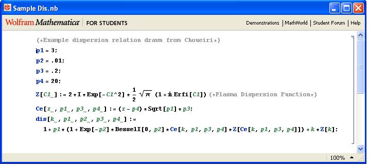
Figure 1 - Sample distribution. Inputing a function in the dispersion relation finder program
Open the file ‘DART.nb’ and type the line shown in the figure below into the box titled ‘function’. The definition of the function must follow the standard Mathematica format, ‘f[k ,w ] := ‘. Also, the function’s name must always be ‘f’. When the function is input, choose minimum and maximum values for \( \omega_\textrm{min} \) and \( \omega_\textrm{max} \) respectively and click ‘enter’. In the left hand side, an ‘argument plot’ will appear with the real values of \( k \) on the x-axis and the imaginary values on the y-axis. At each point in the grid, a line is drawn that makes an angle with the real axis equal to the argument of the function at the corresponding value of \(k\) and \( \omega_\textrm{min} \). Vortices indicate where suspected roots are.
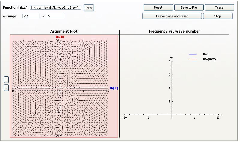
Figure 2 - The 'function' field contains the definition of the dispersion relation of interest. The argument plot for this function is also shown. Zooming in on roots
The next step is to isolate the roots of interest. Click once on the ‘argument plot’. This point will form the corner of a ‘zoom’ box. Move the cursor around and a pink rectangle will follow it. When the desired roots have been highlighted, click again. Within 10-20 seconds, the ‘argument plot’ will be redrawn with boundaries equal to the boundaries of the zoom box. General zooming can also be performed by clicking the ‘+’ and '’ buttons to the left of the argument plot.
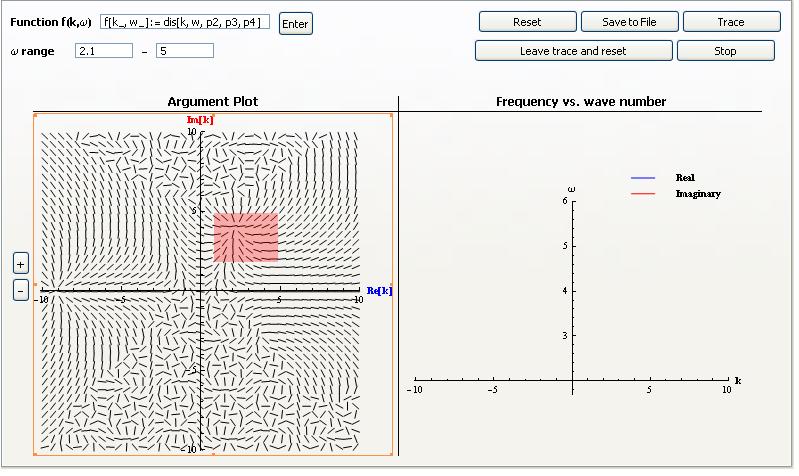
Figure 3 - The highlighted area will form the boundaries of a new 'argument plot'. Tracing
Once the roots of interest have been isolated, click on the ‘Trace’ button. This will initiate the DART algorithm, which will proceed to find the roots in the selected area. Depending on the size of the area and the degeneracy of the roots, this can take anywhere from 5 seconds to 1 minute. Once the roots have been located, the program will start to increment from \(\omega_{\textrm{min}} \) to \( \omega_{\textrm{max}} \) and will trace the migration of the roots. If at any point a root is lost, a new ‘argument plot’ will appear in the left hand column centered at the location of the last known root. It is up to the user to find the vortex corresponding to the lost root, to zoom in on it, and to click ‘Trace’ again. The program will resume where it left off. The location of the root in the complex plane with increasing \( \omega \) is plotted in the left hand window during this process. The real and imaginary parts of \( k \) are depicted vs. \( \omega \) in the right-hand window.
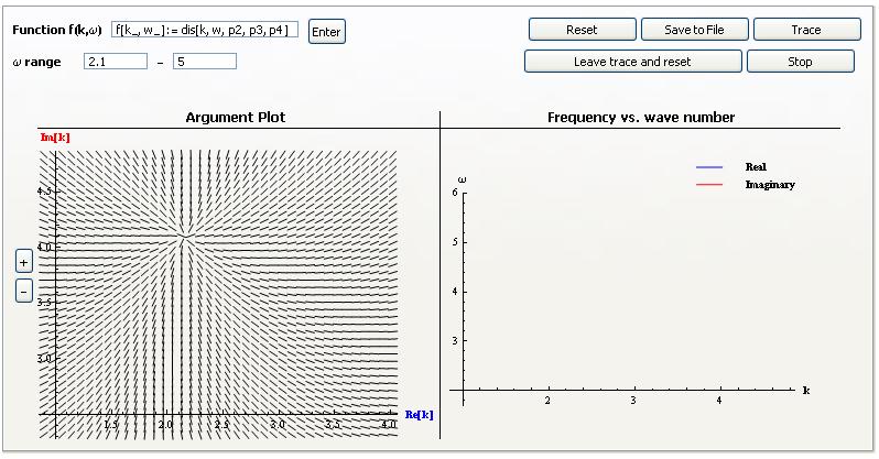
Figure 4 - The zoomed in plot. 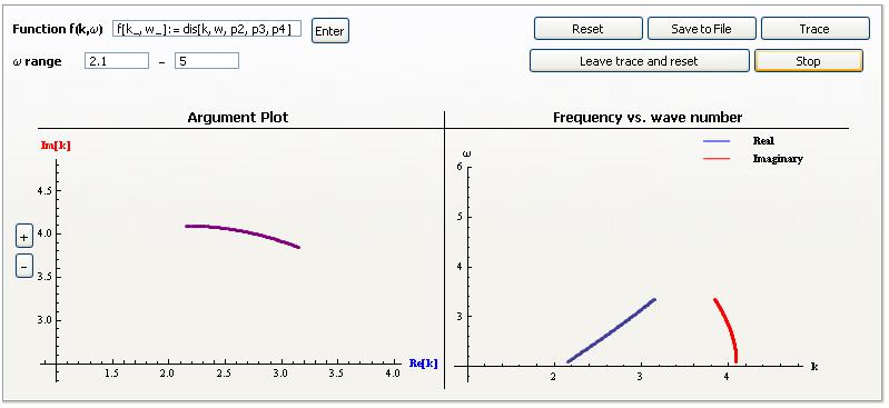
Figure 5 - Stopping and saving
At any point, the user can stop the tracer by pressing ‘Stop’ and save the information to a text file by clicking ‘Save to File’. This will generate a dialog box that allows the user to select the location and name of the file. The output has three columns. The first contains the values of \( \omega \). The second and the third have the real and imaginary values of \(k\) respectively for the root corresponding to \(\omega\). Note: It is possible to trace multiple roots at once with this program. However, the output of the text file will always have three columns, i.e. tracing multiple roots will not generate new sets of columns.
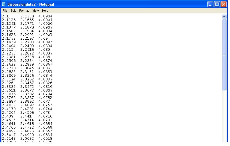
Figure 6 - Sample layout for saved text file. Reset
Once the tracer has completed its task or been stopped, the user can reset the program to display the argument plot at \(\omega_{\textrm{min}}\) again (or a different value if desired). This can be accomplished in two ways. The first is to click ‘reset’. This erases all of the data such that it no longer appears graphically and can no longer be saved. The second method is to click ‘Save trace and reset’. This will reset the program to \(\omega_{\textrm{min}}\) but retain the information on the calculated roots in an array. It will also continue to display the trace in the right hand window. This is beneficial as it allows real time comparison of dispersion relations.
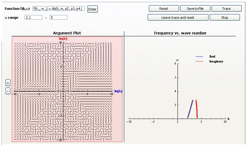
Figure 7 - The trace from the previous run can be saved for the next trace .
This concludes the brief tutorial. The user can use this as a guide for exploring other dispersion relations. It is recommended that the user define a function outside of DART and then input it into the ‘function’ field–just as done in step 2. This will save room in the field and minimize possible errors in defining the function. If there are any any questions or comments, please feel free to contact the author at bjorns@princeton.edu. This is an open source code and free for download and updates.